Apply Analytical Methods

The Replicator Dynamics

The replicator equation describes the dynamics of competing individuals in an infinite population (\(Z\rightarrow \infty\)). It defines the rate at which the frequencies of strategies change over time, following a gradient of selection [1]. A standard form is given by [4]:

\[\dot x_{i} = x_{i} \left(f_i(\vec{x})-\sum_{j=1}^{N}{x_{j}f_j(\vec{x})}\right)\]

where: - \(x_i\) is the frequency of strategy \(i\), - \(f_i(\vec{x})=\Pi_i(\vec{x})\) is the fitness (expected payoff) of strategy \(i\), - \(\sum_{j=1}^{N}{x_{j}f_j(\vec{x})}\) is the average fitness of the population.

EGTtools implements the replicator dynamics for 2-player and N-player games via:

• egttools.analytical.replicator_equation

• egttools.analytical.replicator_equation_n_player

Both functions require a payoff matrix as input. For N-player games, the column index of the matrix corresponds to the group composition, which can be reconstructed using egttools.sample_simplex(index, group_size, nb_strategies).

—

2-Player Games

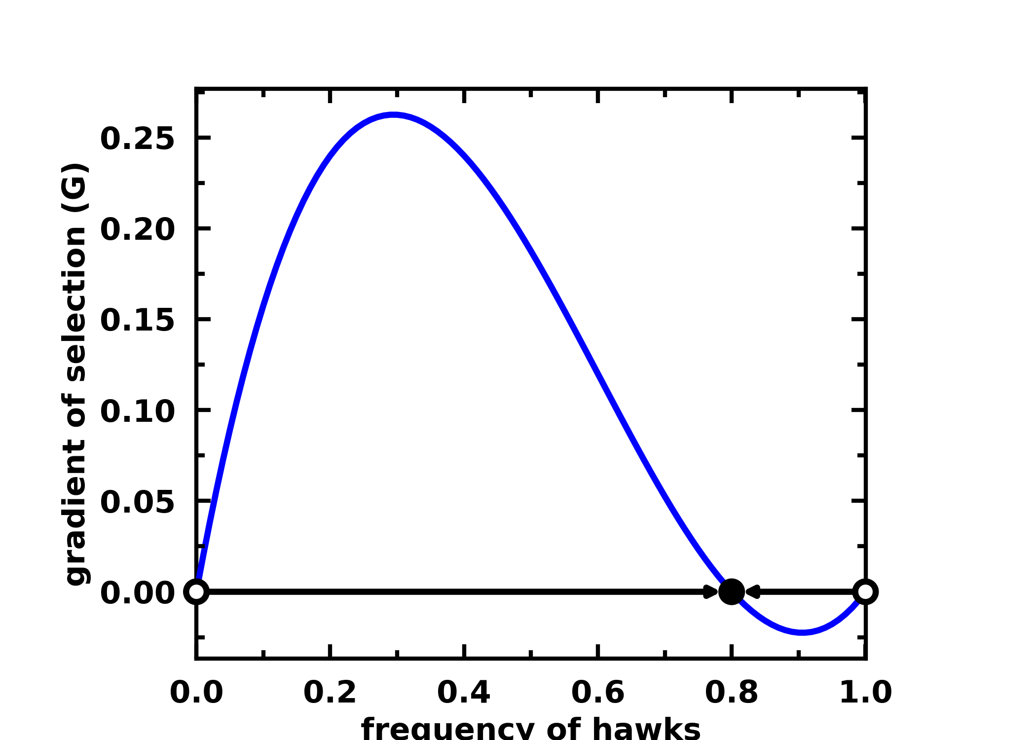
Example for a 2-player Hawk-Dove game:

import numpy as np
import egttools as egt
from egttools.analytical.utils import (calculate_gradients, find_roots, check_replicator_stability_pairwise_games)

payoffs = np.array([[-0.5, 2.], [0., 0]])
x = np.linspace(0, 1, num=101)
gradient_function = lambda x: egt.analytical.replicator_equation(x, payoffs)
gradients = calculate_gradients(np.array((x, 1 - x)).T, gradient_function)

roots = find_roots(gradient_function, nb_strategies=2, nb_initial_random_points=10, method="hybr")
stability = check_replicator_stability_pairwise_games(roots, payoffs)

egt.plotting.plot_gradients(gradients[:, 0], xlabel="frequency of hawks", roots=roots, stability=stability)

You can find additional examples here.

—

N-Player Games

When \(N>2\), groups involve more than two players. Use egttools.analytical.replicator_equation_n_player.

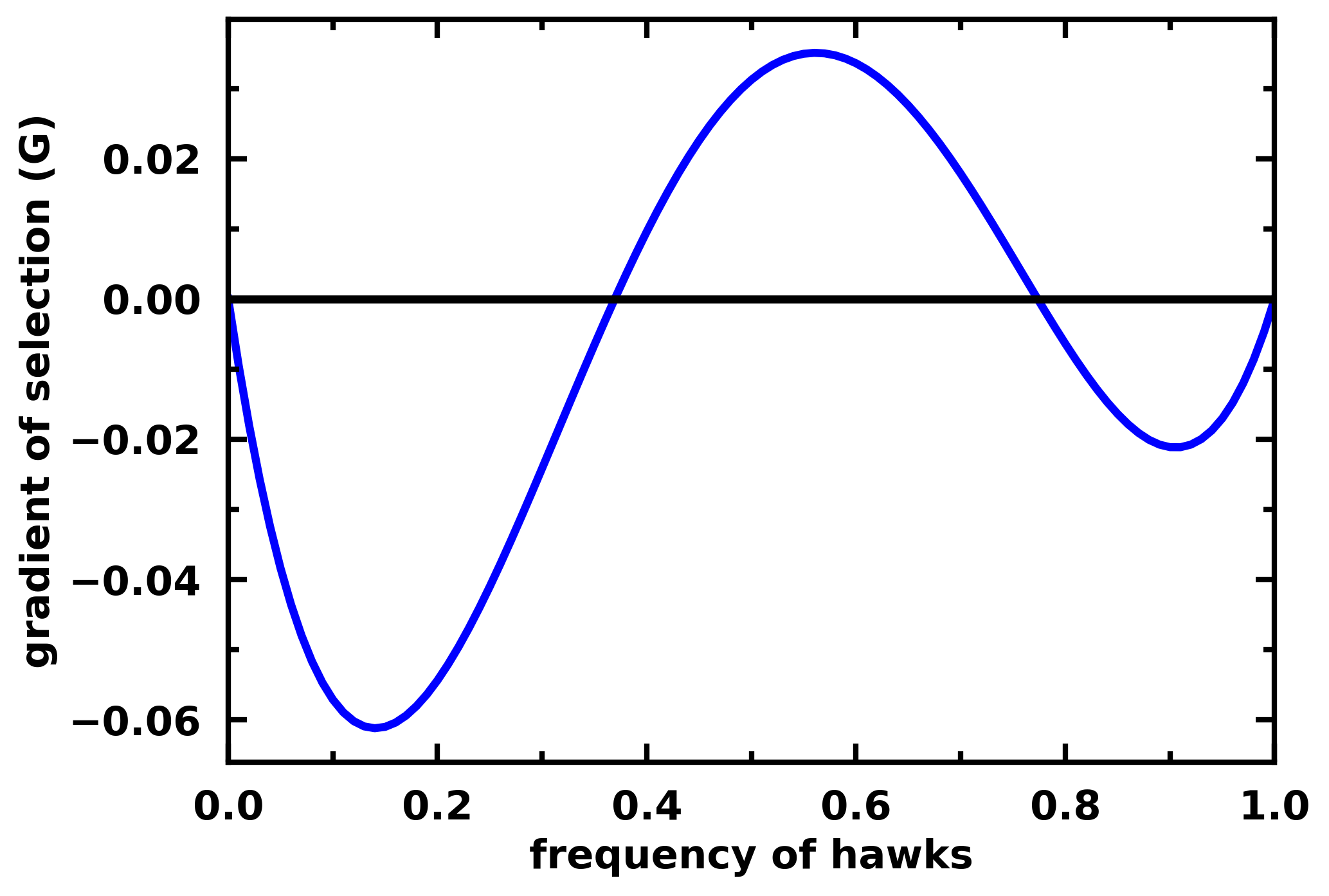
Example for a 3-player Hawk-Dove game:

payoff_matrix = np.array([
    [-0.5,  2. ,  1. ,  3. ],
    [ 0. ,  0. ,  1. ,  2. ]
])

gradient_function = lambda x: egt.analytical.replicator_equation_n_player(x, payoff_matrix, group_size=3)
gradients = calculate_gradients(np.array((x, 1 - x)).T, gradient_function)

egt.plotting.plot_gradients(gradients[:, 0], xlabel="frequency of hawks")

Note

Currently, egttools only supports the analytical stability analysis for 2-player replicator dynamics. Support for N-player stability analysis is planned for version 0.13.0.

—

Stochastic Dynamics in Finite Populations: The Pairwise Comparison Rule

While replicator dynamics assume infinite populations, finite populations introduce stochastic effects [5].

We consider a finite population of \(Z\) individuals interacting in groups of size \(N\), each adopting one of \(n_s\) strategies. Social learning follows the pairwise comparison rule [3, 5, 6]:

At each timestep: - An individual \(j\) considers imitating another individual \(i\), - Imitation occurs with probability following a Fermi distribution:

\[p = [1 + e^{\beta(f_i - f_j)}]^{-1}\]

where: - \(f_i\), \(f_j\) are fitnesses, - \(\beta\) controls selection intensity (low \(\beta\) → random drift; high \(\beta\) → deterministic selection).

Additionally, with probability \(\mu\), individuals may explore strategies randomly (mutation).

The model defines a Markov chain over all possible population states, with state space size:

\[\binom{Z+n_s-1}{n_s-1}\]

[7].

—

Small Mutation Limit (SML)

When mutation is rare (\(\mu \rightarrow 0\)), the evolutionary process simplifies: Populations are mostly homogeneous, with occasional successful invasions by mutants.

The dynamics can be approximated by a Markov chain of size \(n_s\), where transitions are determined by fixation probabilities:

\[\rho_{ji}=\left(1+\sum_{m=1}^{Z-1}\prod_{k=1}^m\frac{T^- (k)}{T^+ (k)}\right)^{-1}\]

[5, 6, 8, 9].

—

Analytical Models in EGTtools

All these analytical results are implemented in:

• egttools.analytical.PairwiseComparison

• egttools.analytical.StochDynamics (legacy, slower)

We recommend using PairwiseComparison, which is optimized in C++. (StochDynamics may be deprecated in future releases.)

Methods in `PairwiseComparison`:

• `calculate_fixation_probability(invading_strategy_index, resident_strategy_index, beta)` Computes the probability that a mutant of a given strategy invades a resident population.

• `calculate_transition_and_fixation_matrix_sml(beta)` Computes the transition matrix and fixation probabilities under the Small Mutation Limit (SML).

• `calculate_gradient_of_selection(beta, state)` Computes the gradient of selection at a given population state (without mutation).

• `calculate_transition_matrix(beta, mu)` Computes the full Markov transition matrix, accounting for selection and mutation.

You can find example usages here and here.

—

Example: Stochastic Dynamics of a Hawk-Dove Game

import numpy as np
from egttools.analytical import PairwiseComparison
import egttools as egt

# Payoff matrix
V, D, T = 2, 3, 1
A = np.array([
    [(V - D) / 2, V],
    [0, (V / 2) - T]
])

# Parameters
nb_strategies = 2
Z = 100
beta = 1

game = egt.games.Matrix2PlayerGameHolder(nb_strategies, A)
evolver = PairwiseComparison(Z, game)

gradients = np.array([
    evolver.calculate_gradient_of_selection(beta, np.array([k, Z - k]))
    for k in range(Z + 1)
])

egt.plotting.indicators.plot_gradients(
    gradients[:, 0], figsize=(6, 5),
    marker_facecolor='white',
    xlabel="frequency of hawks (k/Z)",
    marker="o", marker_size=30, marker_plot_freq=2
)

—

Note

Currently, egttools implements the pairwise comparison rule only. Other processes such as frequency-dependent Moran processes and Wright-Fisher processes are planned.

Note

Support for multiple populations is also under development.